Fundamentals of R
Introduction
There are many tools for analyzing data — in our class combined, I'm sure we've all worked dozens of different platforms in our analysis of data! Some of these, like Microsoft Excel, are likely more familiar to us largely due to their ease of use. But as we do more work with data, we become dissatisfied with their limitations and desire more fine-tuned control.
There are tools to help us achieve this more fine-tuned control. One of these is R, and this is the focus of this unit. R is what we call a statistical computing language. The last word, “language,” indicates that R is a “programming language,” if we use that term loosely. Technically, R is not a language for “programming” in the traditional sense that is understood by other languages like C/C++. Instead, it’s a language for computing things in a way that is statistical. Here, “statistical” refers not only to things like p-values or normal distributions but also to any sort of work with numbers, including cleaning them and analyzing them. In our work together, we will be using this latter understanding of "statistical" broadly across our demonstrations and projects.
In this demonstration, we are going to learn some fundamentals about the R computing language, how to navigate the RStudio interface, and how to create and work with fundamental kinds of data so that we can then be set up to do more interesting things with those data (e.g., analyze or transform them). It is important to note that R does all of the exact same kinds of tasks that other tools can perform when it comes to working with data, but these tasks are expressed through slightly different language. If you have experience with other programming languages, some of these terms will be familiar; if you don't have experience with other programming languages, but you have experience working with data in other tools (e.g., Excel or Tableau), some of the concepts themselves will feel familiar.
Follow along with the guided demonstration below. Fill out the provided template file as you follow along.
An overview of the RStudio interface
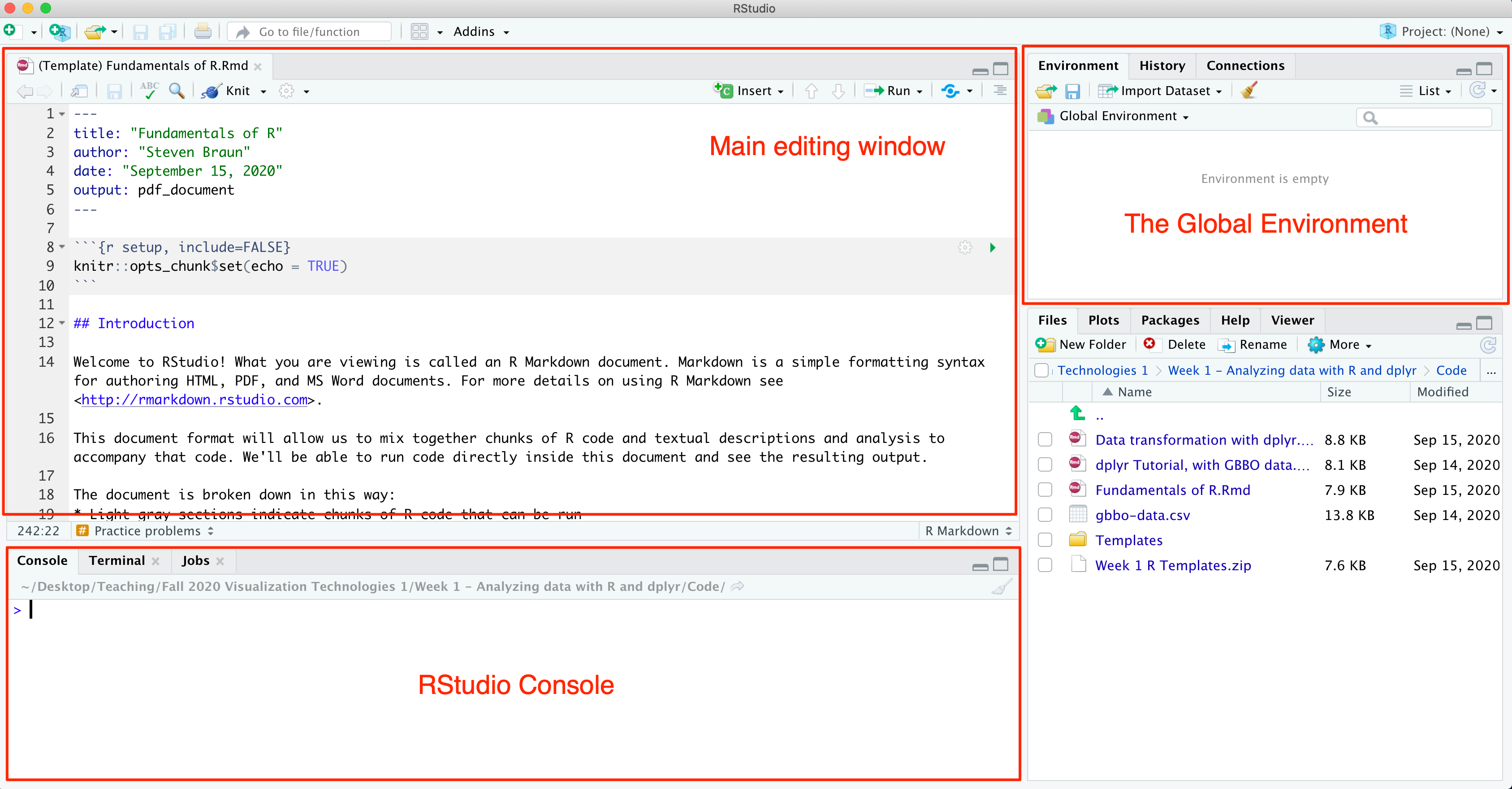
If you open the provided template file in RStudio, you find yourself bombarded with a lot of stuff. This stuff can quickly become overwhelming if you don't know what you're looking at.
Fortunately, there's only a few parts we need to pay attention to. The first of these is located on the bottom part of the window and is called the R Console. This is a place we can interact with the R computing language by typing in commands and instantly seeing what is returned by those commands. We won't use this space much, except to see the outputs of some functions.
At the right side of the screen, we have the Global Environment. This is a place where we can see all the data, values, and objects we have stored in the workspace at any given moment. We'll see what this does for us shortly.
Lastly, and most importantly, we have the main editing window. This is where we will write, edit, and execute our R code to see what that code outputs.
As we move through the following fundamentals, we'll get a sense for what's happening in these areas of the screen.
Using R: Fundamentals
In this next section, we'll encounter the absolutely fundamental ideas that will motivate our work with R in the coming weeks. As you follow along with this demonstration, read each section and examine the code provided on the right. Practice writing the code that you see directly in your template file in the indicated section. Answer any prompts in your file along the way. When you are done, there are some additional practice problems at the very end of the demonstration you may start working with.
An overpowered calculator
In its most basic form, R is an excellent overpowered calculator. For example, R understands many basic kinds of commands and computations, such as the following:
8 + 67 - 53 * 09 / 330 %% 7
In each of the above, the symbols between the numbers indicate specific kinds of calculations. We call them operators. We will use + to add numbers together, - to subtract numbers, * to multiply, and / to divide. The last operator, %%, is for modulo operators: this returns the remainder after division of two numbers. If we place numbers before and after these operators, and then run the code (either by running each individual line or running the code chunk to which it belongs), we'll see what they evaluate to.
We can enter these commands into the RStudio Console one by one, each time pressing the Return key to see the results. When we do this, we see output like this:
> 8 + 6[1] 14
The output we see on the line below gives us the value returned by our input. (For now, ignore the [1] you see.) This works fine when checking one-time-use calculations, but for everything else, we'll want to keep a record of our computations.
Instead of using the console, we'll practice typing these operations in the gray code chunk in the template section labeled 'calculator'. (This can be found in the section under the heading "An overpowered calculator"; notice the comment that say "Type your code for section 'An overpowered calculator' here").
Type each of the commands displayed at right in your template. You can change which numbers to use if you'd like, but the types of computations will stay the same. After you're done, you can either run each line of code one by run, or you can run the entire chunk to see the output.
When working with these commands, order of operations matters! For example, if we want to add two numbers together before multiplying the sum by another number, we must indicate this using parentheses ( ). Likewise, if we want to take one number and divide it by the product of two other numbers, we must indicate that as well. The last couple of examples demonstrate this.
Data types
In the above examples, all of our computations involve numbers, but data can be other types! In R, there are a few key data types that we will care about most; every value we use will be one of these types.
Numeric data types include values that are numbers. This includes both integers and decimal values, and positive or negative numbers. Character types include strings of letters, words, or phrases. We indicate a character type by placing the value between quotation marks. We can use single or double quotation marks, but regardless of which we choose, we must use matching types on both sides. (Notice in the examples that 'blue' uses single quotation marks while "banana" uses double quotation marks.)
The last major data type in R is the Logical type. In R, this includes the values TRUE, FALSE, and NA, which refers to a value that is missing or doesn't exist.
Assigning data to objects
In the above examples, we're purely creating values that exist only momentarily at the instant we 'execute' them. When we want to store a value somewhere for later use in our code (e.g., if we want to use the same value in many places without having to type the same value over and over again), we can assign the value to an object. An object is basically a name that we choose that holds the value we want to use in other places. We accomplish this by using the assignment operator, which looks like a left-pointing arrow <-. In R, an object behaves just like a variable in other programming languages, but the word 'variable' is reserved for a different meaning in R specifically, so we won't use that word here.
Any time we name a new object, it gets stored in the Global Environment. But we must always remember to actually run the code that define our objects, otherwise the environment won't know they exist! After you've defined an object, make sure to run the code chunk it's located in. You should see an updated environment that looks like this:
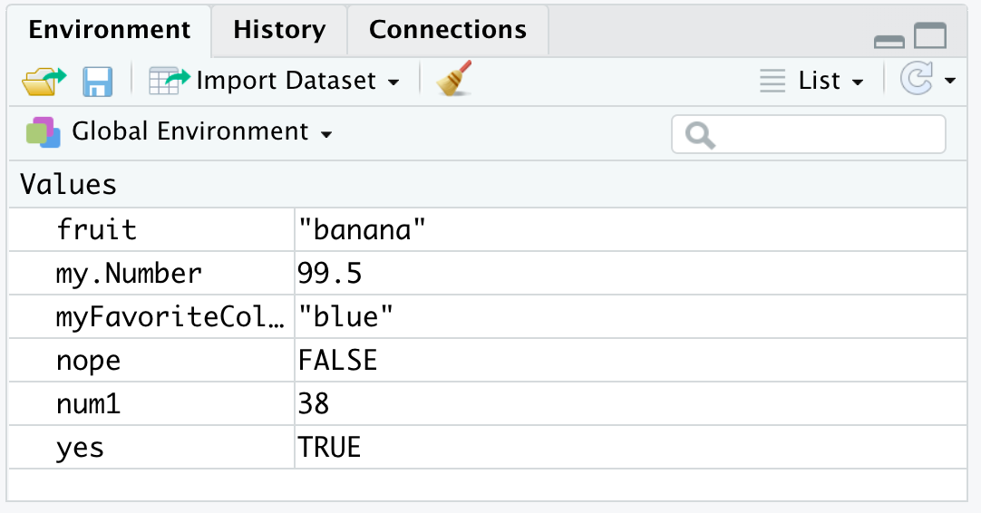
We can use any named objects that are stored in the environment in other expressions, as long as we refer to them exactly in the same way they've been defined. This means any references must match exactly the original object name in capitalization, spelling, and punctuation.
Something we need to be careful about is keeping track of the data types of our objects. For example, if we try to add two objects together that both refer to numeric data types, then we will get a number back; if we try to add one object whose data type is numeric and another object whose data type is character, then we will get an error, such as when we try to do this:
Error in myFavoriteColor + fruit : non-numeric argument to binary operator# What happens when you try to use + with two Character values?myFavoriteColor + fruit
This is R's obscure way of telling us "You're trying to add two different data types together, but I expected both values to be numbers!"
Performing comparisons
In addition to performing arithmetic with values, we can also compare them. Using comparison operators, we can test for things like equality or inequality, or if one value is greater or less than another value. We can use these operators for any kind of R data type, including numbers, characters, and logical values.
Every comparison operator returns a value of TRUE or FALSE, depending on whether the comparison passes the given test. The following comparison operators are especially useful:
A > B: ReturnsTRUEif the value of A is strictly greater than the value of B (andFALSEotherwise)A < B: ReturnsTRUEif the value of A is strictly less than the value of BA >= B: ReturnsTRUEif the value of A is greater than or equal to the value of BA <= B: ReturnsTRUEif the value of A is less than or equal to the value of BA == B: ReturnsTRUEif the value of A is equal to the value of BA != B: ReturnsTRUEif the value of A is NOT equal to value of B
For the most part, these comparisons work as expected for numbers, but we must be careful about working with character data types. With character values, the equality and inequality operators are strict, meaning that equality is measured only if both characters match exactly in spelling, capitalization, and punctuation. Strangely, we can sometimes coerce a value of TRUE from comparing a numeric against a character value, such as in this example:
[1] TRUE# Be careful when comparing numbers!15 == "15"
Technically, both values are different in type, but they evaluate to the same apparent value of '15'. This is called type coercion, which means a value of one data type gets coerced to a different data type depending on the context in which it is used. Be careful! This can happen behind the scenes without us knowing it.
Vectors of data
All of the above examples deal with atomic data types, i.e., singular values. Most of the time, we'll be more interested in performing calculations on collections of data. In R, a collection of data is called a vector. (The concept of vectors is very similar to the concept of arrays in other programming languages, but again, we won't be using that word.)
We declare a vector of values by using a function in R called c(), and place our values inside the parentheses separated by commas. Importantly, in R, all values in a vector MUST be the same type. In other words, we can have a vector of numeric values, or a vector of character values, but we can't have a vector of mixed character and numeric values.
If we do happen to mix together data types in a vector, we might get lucky and see no error. But when this happens, beware! This means that type coercion is happening again somewhere. In this example, since the numeric values of 8 and 93 can be coerced into character types, all values in the vector get coerced into character types. This can cause us serious problems later in our code, so it's best to catch these issues early.
Built-in functions
Once we have vectors of data, that's when the real fun starts because we can use built-in functions to perform calculations on those vectors. In R, there are many such functions that we can invoke by a single command to do many common kinds of analyses, such as summing a vector of values, finding an average value, or determining the range of values from a min and max value. Some of these are demonstrated here.
Most functions have optional parameters that we can pass along into it to customize how the function will be used. To see more information about how to use a function, we can use the ? symbol followed by the name of the function (with no space). If we execute this from the console or our script, information pops up in the bottom-right section of the screen labeled 'Help'. This is an extremely useful part of RStudio.
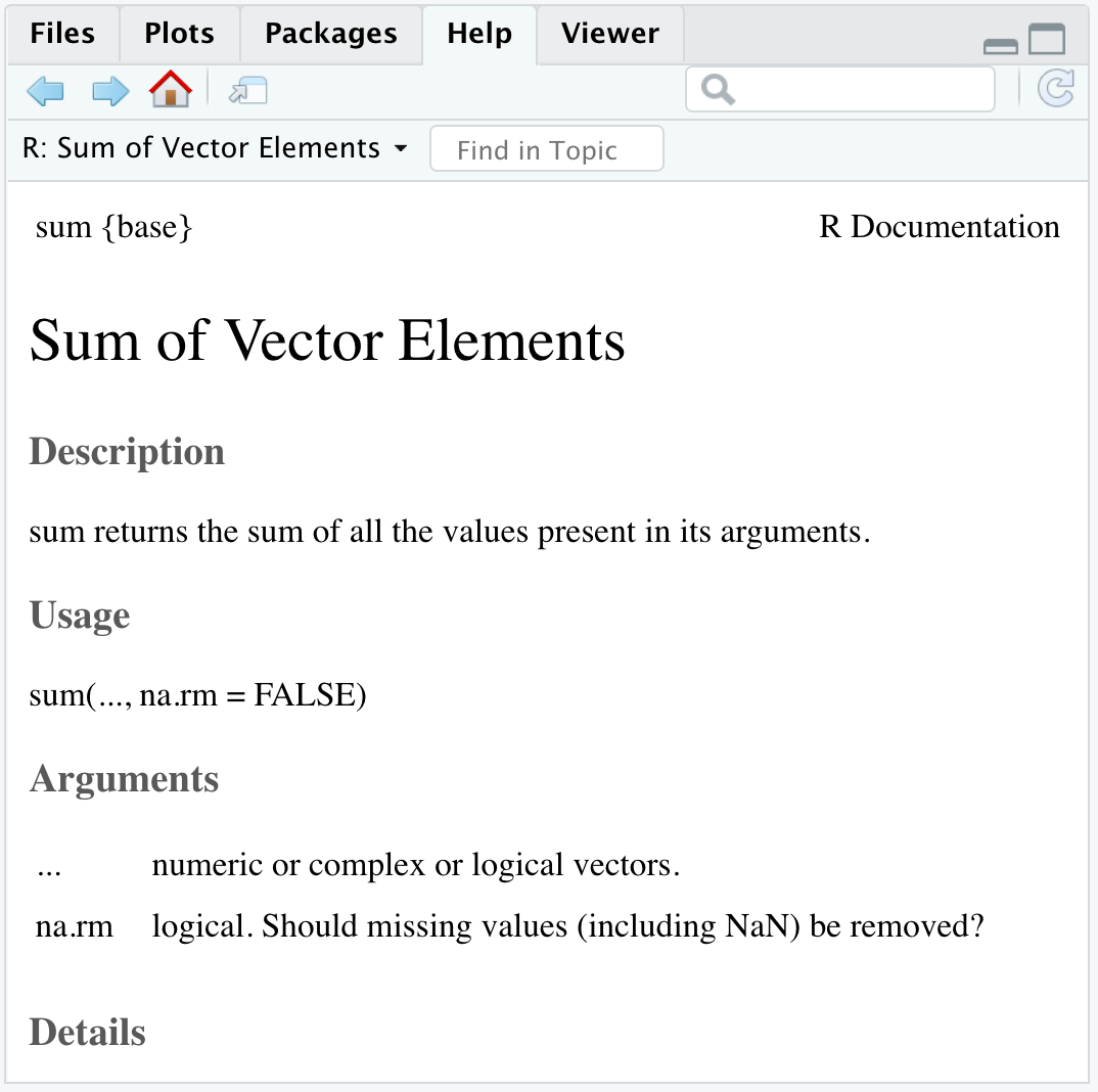
?sum.
sd() do? How would you find this out? Use this function on the vector named 'my.data' here.Data frames
Finally, we've arrived at the most useful data structure of all in R: tables of data. In R, a table of data is called a data frame. Data frames will be most useful to us, since we'll be wanting to load in entire data sets from CSV in order to transform or analyze them. Whenever we load in a CSV file, it will be converted into a 'data frame.'
Data frames have certain terminology associated with them. Each column in a data frame is called a variable. Each row is called an observation. We'll be using these terms for very specific purposes in R.
R has many built-in data sets that we can inspect and explore. Here, we'll investigate the built-in data set named trees. (You can see more available data sets by running the command data().) We can pass the name of this data frame into the View() function to see what's inside. You'll notice it has a few variables: Girth, Height, and Volume.
If we want to view or do something with one variable of interest, we can subset it using the $ symbol, as shown. We can use this to take a single column and pass it into other functions, like mean().
More practice
Once you're done working through the demonstration above, work through the following practice problems to reinforce your learning. Make sure to type your responses in your template file in the space given.
- Name at least 5 new objects (of your choice). Assign a different value to each object. At least one object data type must be numeric, character, and logical.
- Using your named objects from (1), create a minimum of 4 expressions using each of the following operators at least once: +, -, *, /
- Create a new object whose value is a vector of numeric values.
- Using the functions sum(), mean(), max(), and min(), calculate the total sum, average value, and range of values in your vector from (3).
-
Choose another built-in data frame in R (using
data()). Load that data set by name. Subset a single column from the data frame using $, and assign that subsetted column to a new object that you name.