Loading dplyr and an example data set

In order to use any library in R, we must first load it into the R workspace environment. And before we can even do that, we need to install it on our computers. This is true of dplyr: we don't by default have this library installed on our computers unless we explicitly tell RStudio to do so. As we do more work with R, it will become commonplace to load and unload libraries for different reasons, and next week, we'll encounter a collection of libraries that will make this work even easier.

In R, we can use the function install.packages() to download and install any package/library we want to work with. Inside the parentheses, we will place the name of the desired library in quotation marks. We only ever need to install a library once on our computers to use it repeatedly over multiple R sessions.

The package we will download and install is called dplyr, indicated in the parentheses. If you run this line of code, you should see an output in the R console that looks like this:

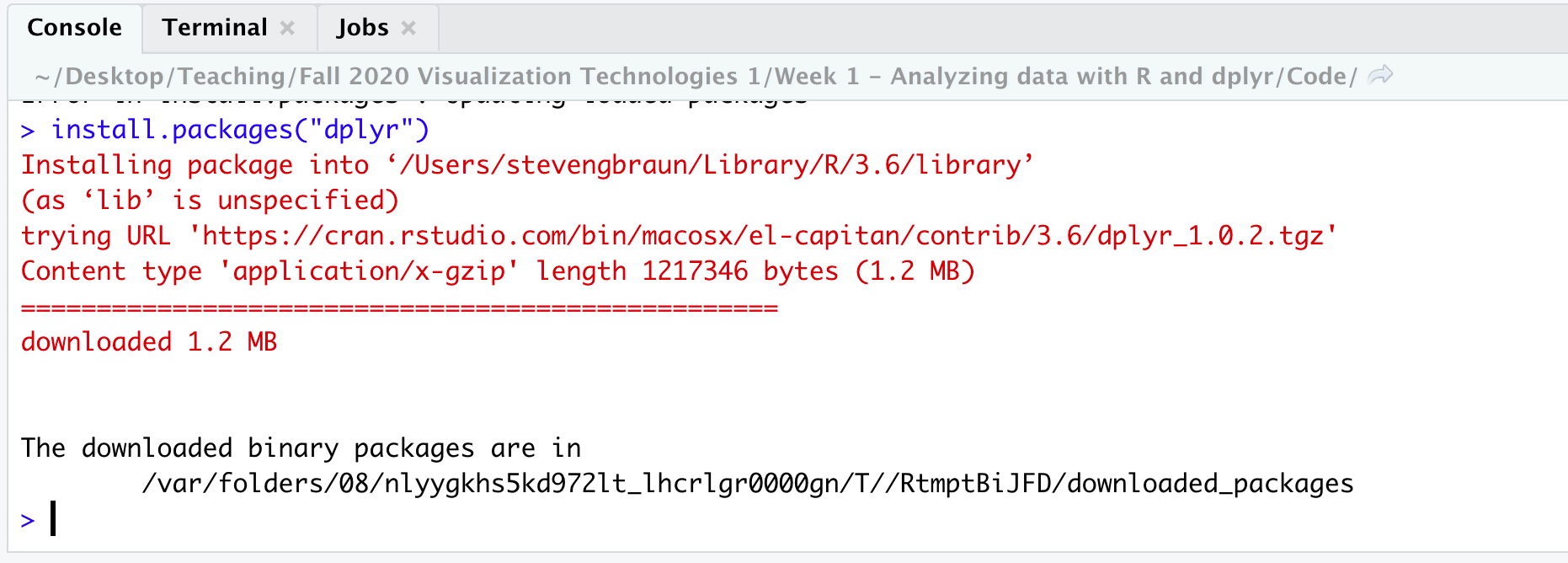
After we have installed the package, it doesn't by default get activated so we can use it. We will need to load it into our current workspace. To do that, we need to use the function library(). (Notice that when we pass in the name of the library here, we don't use quotation marks, even though we did when we used install.packages().) Whenever we want to use a library like dplyr, we will always need to load it into the workspace every time we need it. Both of these functions are demonstrated in the code chunk provided.

Make sure to run the whole code chunk, or each line individually, in order to install and then load in the dplyr library.

Choosing our data set

Once we have dplyr installed and loaded, we can now start to use it. For this demonstration, we are going to explore one of R's built-in data sets that's already loaded into the workspace. Here, we'll work with one of the datasets built into dplyr specifically: starwars.

Just like we saw in our basic R demonstration, we can directly refer to this library by name. In our demonstration, though, we're going to assign the original data name to a new object name, for ease of reference and use later on.

Before proceeding, let's look at the data frame to see what's inside. In addition to the View(), function, we can use other R functions for seeing the data, including head() to only display the first few rows, or summary() to view a statistical summary of all variables. Try running these to see what kind of output they produce.

dplyr verbs

Now that we have our data, we can get to the good stuff: working with dplyr "verbs". In dplyr, these verbs are functions that perform common data transformation tasks using code that is simpler than what the equivalent code in base R would be to do the same thing. In each section that follows, a verb will be introduced, and you'll be invited to see the outputs they yield.

The command structure for all dplyr verbs is as follows:

VERB(DATAFRAME, ARGUMENTS...)

Note that every dplyr function returns a data frame, but it does not automatically write over any data frames that are stored inside of objects! So if we make changes we want to use elsewhere in our code, we need to capture the outputs in a new object name.

The next sections introduce each major verb function one at a time.

select: Pick columns by name

A common task when working with data is to reduce the amount of variables we are looking at, such as when we don't need to use an entire data set. If we only want to look at or use specific columns of interest (not all the columns), we can use select().

As with every dplyr verb, the first argument to this function will always be the data frame we want to operate on. (Here, our starwars data frame, which we've stored in an object named 'data'.) The arguments that follow for this verb are all of the columns we want to keep in the data set. We separate these column names by commas. Column names must exactly match the names in the data frame.

We can select one or more columns from a data frame with this verb. If we want to select contiguous columns, we can do so using the colon operator. Run this line of code and see what it outputs.

Again, remember that these verbs don't change the original data set!

filter: Keep rows matching criteria

We use the filter() function to selectively retrieve (or filter) only those observations (rows) that meet criteria we specify. If we only want to see rows that pass a certain condition, we would use this verb.

In the first example at right, we are using a comparison operator to return all rows where the value of 'mass' is greater than or equal to 80. If we want to filter based on multiple conditions, we can separate those conditions using commas. When we do this, all conditions must be met simultaneously in order for a row to be returned. (This is equivalent to the Boolean AND function). In this example, we are using this verb to filter those rows in the data where 'mass' is greater than or equal to 80 and 'eye_color' is equal to 'blue'.

The commas indicate Boolean AND operations by default. If we want to filter rows based on one criterion or another one, we can separate those conditions using the vertical pipe (|) operator. We can combine AND with OR operations in the same line of code. In this example, we are filtering rows where 'mass' is greater than or equal to 80, and where 'eye_color' is 'blue' or 'eye_color' is 'brown'.

Definining several OR conditions can get tedious. To simplify this, we can use the special operator %in%. On the left of this operator, we specify the name of a variable (column); on the right, we supply a vector of values. If the value of the given variable matches one of the values on the right-side (in the vector), then the row gets returned.

Another reminder: The verbs above do not modify the original data set! If you look at 'data' again, you'll see that the original data still persist; nothing has been filtered. To store the results of a dplyr function, you must reassign to an object:

humans.droids <- filter(data, species %in% c("Human", "Droid"))

With this, we can now use this filtered data set for any purpose.

arrange: Reorder rows

Another common operation is sorting data. When we want to sort our data, for example from smallest to largest, we can use arrange().

This verb is pretty straightforward: the argument(s) you supply are any valid names of columns in the data set. The function will rearrange the order of the rows based on the value of that column. By default, this function sorts in ascending order by value, but we can sort in descending order using the special helper function desc() inside of the call to arrange() itself.

mutate: Add new variables

In the examples so far, we haven't modified the data structure. When we want to create new variables, such as calculations based on existing variables, we can use mutate(). Note that any new variables we create are automatically placed at the end (far right column) of a data frame.

To create a single new column in a data frame, we use the following formula:

mutate(DATAFRAME, NEW COLUMN NAME = VALUE)

We can name the new column anything we want, following standard naming requirements. The value of the new column will be computed individually for each row and added to the data frame. Most helpfully, we can refer to existing column names in that calculation. For example here, we are creating a new column named 'weight.in.pounds' whose value will be the value of the 'mass' column converted into pounds. The 'mass' column already exists, and here we can reference it directly by name.

We can do lots of interesting things with mutate(), such as the example with lengths() here. What is this doing to our data frame?

summarize: Reduce variables to values

Finally, when we want to summarize a data set, such as find the mean value of a specific column, we can use summarize(). The structure of this verb is very similar to mutate(), but instead of calculating a new value for each individual row, summarize() reduces a calculation down to a single value.

In the first example, we are creating a new variable named 'avg.height' whose value is the average height of the entire column named 'height'. But this gives us an unexpected output!

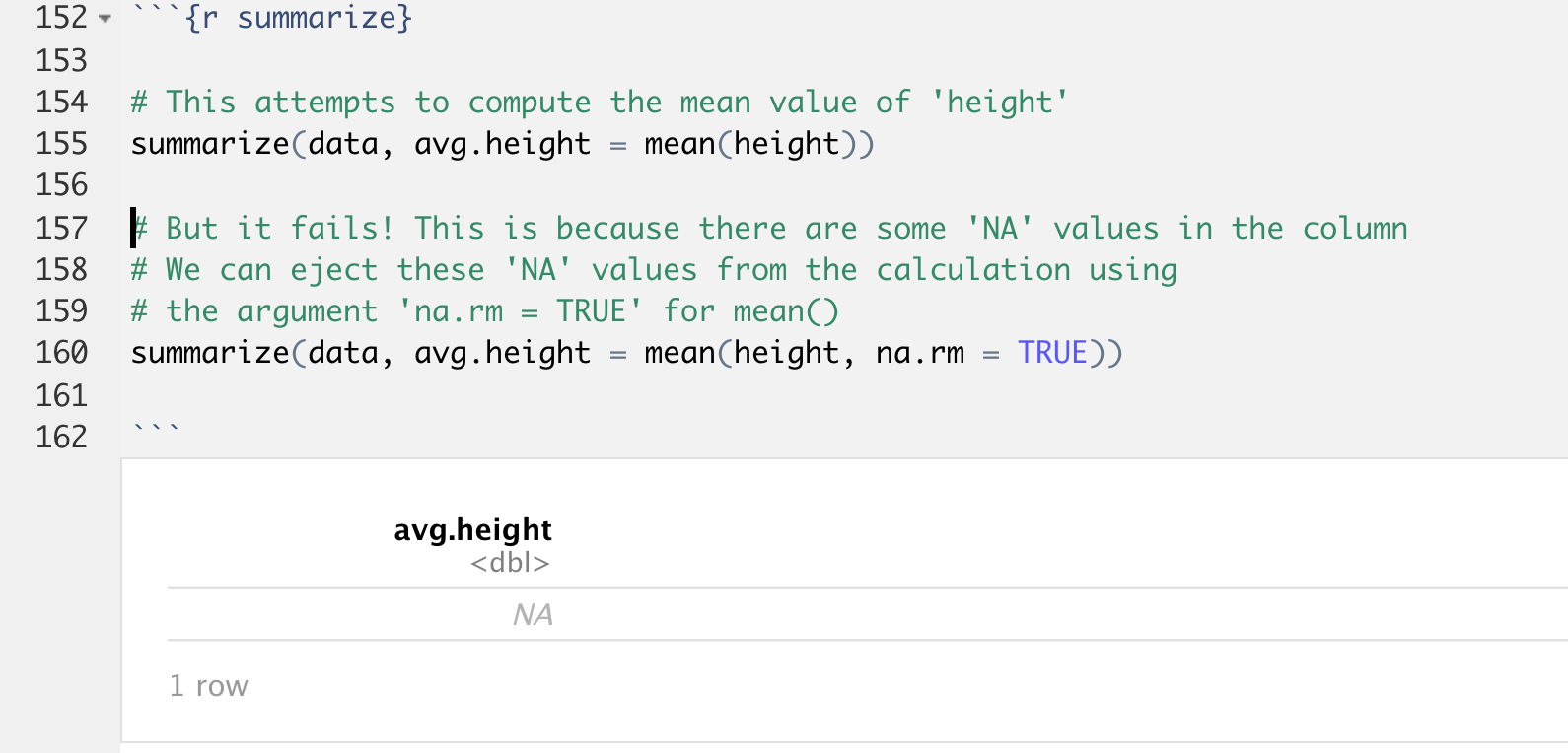
Instead of seeing a number, we see a value of NA. The source of this problem is our mean() functions. It turns out there are some missing values in our 'height' column, and this function doesn't know what to do with those values, so it silently fails.

We can fix this problem by adding another argument to mean(), by specifying na.rm = TRUE. This tells the function to ignore any missing values in the calculation of the mean. Try running this now and see what happens.

"Piping": using chained functions

Most of the time, we'll want to do multiple transformations in sequence: select first, then filter, etc.

Instead of doing all of these tasks individually and nesting functions, we can use the pipe operator in dplyr.

The pipe operator, %>%, allows us to take the output of a preceding function and use it as the input of the next function. When we use the pipe, the first argument of the function that follows the pipe is assumed to be the output of the previous function.

For example, examine the following:

data %>% select(name, species, eye_color, mass)

In the above example, the data frame named 'data' is piped into the select() function, which assumes now that the first argument (the data set) is 'data'. This statement is then read as "Select the columns 'name', 'species', 'eye_color', and 'mass' from 'data'". If we pipe this further:

data %>%
    select(name, species, eye_color, mass) %>%
    filter(mass > 100)

Now the order of commands is this:

• Take the data frame named 'data' and pipe it into select()
• Using select(), only grab the columns named 'name', 'species', 'eye_color', and 'mass'
• Take that subsetted data frame and pipe it into filter()
• Using filter(), only return those rows where the value of 'mass' is greater than 100

It is important to note that the pipe operator (%>%) ONLY works with dplyr, so make sure you have loaded dplyr with library() before using it in your code!

Try typing and running the expressions you see at the right in your template file. What do you see as the output? Are you surprised by anything you see? Are these expressions working as expected?

group_by: Group observations by value

Piping is especially useful when we want to do a series of actions on a grouped data set. The last important dplyr verb, group_by(), enables us to group like observations based on the value of a variable we specify, which we can then use for more advanced computations. This is especially helpful when using summarize().

In the examples at right, notice that if we use group_by() by itself, we don't see anything change in the data frame. That's because nothing is actually changing in the structure of the data, just how dplyr is interacting with it. To see anything useful, we will need to pipe the output of group_by() into another verb. Consider the examples at the right. Type each one and make a prediction about what you will see. Are you surprised by anything?